The transformer model was a complete revolutionizer in the field of Natural Language Processing by utilizing self-attention mechanisms, enabling parallel processing of input sentences. Unlike RNNs, which process sequentially, Transformers handle entire sequences at once, making them faster and more scalable for large datasets. Its unique architecture includes multi-head attention and positional encodings, allowing the model to capture relationships between words regardless of their positions in the text sequence. Transformers excel in tasks like translation, summarization, and most famously question answering, forming the foundation for models such as GPT and BERT.

In this article, we will dive deep into every intricacy of the Transformer model including: Positional Encoding, Attention Mechanisms, Masking, Encoder Layer, and Decoder Layer.

By the way, this is a must-read for anyone learning the attention-based models: Attention Is All You Need

I have also tried to implement the Transformer from scratch using PyTorch: The-Transformer-Model

1. Positional Encoding

In sequence to sequence task, the relative order of your data (the ordering of words in sentences) is extremely important to derive the semantic meaning of the inputs. And while training sequential neural networks such as RNN, we feed our inputs into the model in order. Therefore, information regarding the order of data is fed automatically into the model. However, in the Transformer network using multi-head attention, we feed the data all at once. And while this significantly reduces training time, there is absolutely no information about the order of our data. That is when Positional Encoding comes into play. We can encode the positions of your inputs and pass them into the network using these sine and cosine formulae:

PE_{(pos, 2i)}= sin\left(\frac{pos}{{10000}^{\frac{2i}{d}}}\right)

PE_{(pos, 2i+1)}= cos\left(\frac{pos}{{10000}^{\frac{2i}{d}}}\right)

Where $d$ is the dimension of the word embedding and positional encoding.

We can intuitively think positional encodings as a feature that contains information about the relative ordering of words. The sum of the positional encoding and word embedding is ultimately what is fed into the model. If you just hard code the positions in, say by adding a matrix of 1's or whole numbers to the word embedding, the semantic meaning is distorted, since the word embedding is distorted.

Conversely, the values of the sine and cosine equations are small enough (between -1 and 1) that when you add the positional encoding to a word embedding, the word embedding is not significantly distorted, and is instead enriched with positional information. Using a combination of these two equations helps your Transformer network attend to the relative positions of your input data.

1.1 Sine and Cosine Angles

Although the sine and cosine positional encoding equations use different indices (2i for sine and 2i+1 for cosine), both share the same underlying term:

\theta(pos, i, d) = \frac{pos}{10000^{\frac{2i}{d}}}

Example:

PE_{(pos, 0)} = \sin\left(\frac{pos}{10000^{\frac{0}{d}}}\right) \quad\text{and}\quad PE_{(pos, 1)} = \cos\left(\frac{pos}{10000^{\frac{0}{d}}}\right)

Here, solving 2i = 0 or 2i+1 = 1 both give (i = 0), meaning the angle is identical for the sine–cosine pair.
This pairing occurs across all dimensions, forming matched sine and cosine curves — a property central to how positional encodings preserve relative position information.

def get_angles(position, k, d_model):
    i = k // 2
    angle_rates = 1 / np.power(10000, (2 * i) / np.float32(d_model))
    
    return position * angle_rates

1.2 Sine and Cosine Positional Encodings

def positional_encoding(positions, d):
    # initialize a matrix angle_rads of all the angles
    angle_rads = get_angles(np.arange(positions)[:, np.newaxis],
                          np.arange(d)[np.newaxis, :],
                          d)
 
    # Apply sin to even indices in the array; 2i
    angle_rads[:, 0::2] = np.sin(angle_rads[:, 0::2])
 
    # Apply cos to odd indices in the array; 2i+1
    angle_rads[:, 1::2] = np.cos(angle_rads[:, 1::2])
 
    pos_encoding = angle_rads[np.newaxis, ...]
 
    return tf.cast(pos_encoding, dtype=tf.float32)

Let's try visualizing this: Each row represents a positional encoding, and none of the rows are identical. The wavy curves of sine and cosine has enabled us to create a unique positional encoding for each of the words.

2. Attention Mechanisms

Attention models constitute powerful tools in the NLP practitioner's toolkit. Like LSTMs, they learn which words are most important to phrases, sentences, paragraphs, and so on. Moreover, they mitigate the vanishing gradient problem even better than LSTMs.

We will explore four ways of attention: Self-attention, causal (masked) attention, bi-directional self-attention, cross-attention and multi-head attention.

2.1 Self-attention

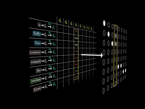
Self-attention, also known as scaled dot-product attention, is a core mechanism in Transformers that allows the model to capture dependencies between tokens within a sequence. In self-attention, each token in the input sequence attends to all other tokens (including itself) to determine which other tokens it should focus on. This seemingly simple operation would return rich, attention-based vector representations of the words in your sequence. Self-attention can be mathematically expressed as:

Attention(Q, K, V) = softmax(\frac{QK^T}{\sqrt{d_k}})V

where $Q$ , $K$ , and $V$ represent the query, key, and value matrices respectively.

def dot_product_attention(q, k, v, mask, scale=True):
    # Multiply q and k transposed.
    matmul_qk = tf.matmul(q, k, transpose_b=True)  # (..., seq_len_q, seq_len_k)
 
    # scale matmul_qk with the square root of dk
    if scale:
        dk = tf.cast(tf.shape(k)[-1], tf.float32)
        matmul_qk = matmul_qk / tf.math.sqrt(dk)
 
    # add the mask to the scaled tensor.
    if mask is not None:
        matmul_qk = matmul_qk + (1. - mask) * -1e9
 
    # softmax is normalized on the last axis (seq_len_k) so that the scores add up to 1.
    attention_weights = tf.keras.activations.softmax(matmul_qk)
 
    # Multiply the attention weights by v
    attention_output = tf.matmul(attention_weights, v)  # (..., seq_len_q, depth_v)
 
    return attention_output

With a basic dot product, we capture the interactions between every word embedding in the query and every word in the key. If the queries and the keys (hence the values) belong to the same sentence, this is Bi-directional (sometimes also called fully-connected) self-attention.

2.2 Causal Attention

If the queries and the keys (hence the values) belong to the same sentence, but we only consider words that come before the current ones, this is causal attention.

def causal_dot_product_attention(q, k, v, scale=True):
    mask_size = q.shape[-2]
    mask = tf.experimental.numpy.tril(tf.ones((mask_size, mask_size)))  
    return dot_product_attention(q, k, v, mask, scale=scale)

2.3 Multi-head Attention

Multi-head attention is an extension of self-attention. Instead of performing the attention calculation once, multi-head attention splits the input into multiple smaller 'heads' and performs separate self-attention calculations in parallel on each. Each head learns different aspects of the input relationships.

Multi-head attention allows the model to represent even more complex relationships in the data. By attending to different parts of the sequence in parallel, it can capture multiple types of dependencies between tokens.

In case Multi-head attention is difficult to grasp, try referring to this gem videos (at 19:19 timestamp):

3. Masking

Masking is another essential building blocks of the transformer. There are two types of masks that are useful in the Transformer Model: the padding mask and the look-ahead mask.

This is the formula for the attention after applying the mask:

\text{Attention}(Q, K, V) = \operatorname{softmax}\left( \frac{Q K^{T}}{\sqrt{d_{k}}} + M \right) V

where $M$ is the optional mask you choose to apply.

Essentially, when feeding sequences into a transformer model, they need to be of uniform length: Sequences longer than the maximum length are truncated and sequences shorter than the maximum length are padded with zeros.

In the attention layers, the zeroes (padding) will typically disappear due to mathematical operations. However, it is desirable that the model should only attend to the actual data rather than the paddings.

The padding mask a boolean mask that indicates which elements in the sequence should be attended to (1) and which should be ignored (0). The mask is used to set the values of the vectors corresponding to the zeros in the initial sequence to a very large negative number (close to negative infinity, -1e9). This ensures that when the softmax function is applied, the padded elements (zeros) do not affect the attention scores.

For example, we have the input vector is [87, 600, 0, 0, 0] and the mask is [1, 1, 0, 0, 0]. When your vector passes through the attention mechanism, you get another (randomly looking) vector, let's say [1, 2, 3, 4, 5], which after masking becomes [1, 2, -1e9, -1e9, -1e9], so that when you take the softmax, the last three elements (where there were zeros in the input) don't affect the score.

def create_padding_mask(decoder_token_ids):
    seq = 1 - tf.cast(tf.math.equal(decoder_token_ids, 0), tf.float32)
    return seq[:, tf.newaxis, :]

If you multiply (1 - mask) by -1e9 and add it to the sample input sequences, the zeros are essentially set to negative infinity. Notice the difference when taking the softmax of the original sequence and the masked sequence here:

Softmax of non-masked vectors:
tf.Tensor( [[[7.2959948e-01 2.6840466e-01 6.6530862e-04 6.6530862e-04 6.6530862e-04]] 
			[[8.4437370e-02 2.2952458e-01 6.2391245e-01 3.1062771e-02 3.1062771e-02]]
			 [[8.3392531e-01 4.1518696e-02 4.1518696e-02 4.1518696e-02 4.1518696e-02]]], shape=(3, 1, 5), dtype=float32)
 
Softmax of masked vectors: 
tf.Tensor( [[[0.73105854 0.26894143 0. 0. 0. ]] 
			[[0.09003057 0.24472848 0.6652409 0. 0. ]]
			[[1. 0. 0. 0. 0. ]]], shape=(3, 1, 5), dtype=float32)

The look-ahead mask follows similar intuition. In training, you will have access to the complete correct output of your training example. The look-ahead mask helps your model pretend that it correctly predicted a part of the output and see if, without looking ahead, it can correctly predict the next output.

For example, if the expected correct output is [1, 2, 3] and you wanted to see if given that the model correctly predicted the first value it could predict the second value, you would mask out the second and third values. So you would input the masked sequence [1, -1e9, -1e9] and see if it could generate [1, 2, -1e9].

def create_look_ahead_mask(sequence_length):
    """
    Returns a lower triangular matrix filled with ones
    Arguments:
        sequence_length (int): matrix size
    Returns:
        mask (tf.Tensor): binary tensor of size (sequence_length, sequence_length)
    """
    mask = tf.linalg.band_part(tf.ones((1, sequence_length, sequence_length)), -1, 0)
 
    return mask

4. The Encoder

The Transformer Encoder layer pairs self-attention and convolutional neural network style of processing to improve the speed of training and passes $K$ and $V$ matrices to the Decoder. Our Encoder looks something like this: The input sentence first passes through a multi-head attention layer, where the encoder looks at other words in the input sentence as it encodes a specific word. The outputs of the multi-head attention layer are then fed to a feed forward neural network. The exact same feed forward network is independently applied to each position.

4.1 Feed Forward Neural Network

def FullyConnected(embedding_dim, fully_connected_dim):
    model = tf.keras.Sequential([
        tf.keras.layers.Dense(fully_connected_dim, activation='relu'),  # (batch_size, seq_len, d_model)
        tf.keras.layers.Dense(embedding_dim) 
    ])
 
    return model

4.2 The Encoder Layer

Now we pair multi-head attention with the FFNN built above. We will also include residual connection and layer normalization to help speed up training.

class EncoderLayer(tf.keras.layers.Layer):
    """
    The encoder layer is composed by a multi-head self-attention mechanism,
    followed by a simple, positionwise fully connected feed-forward network.
    This architecture includes a residual connection around each of the two
    sub-layers, followed by layer normalization.
    """
    def __init__(self, embedding_dim, num_heads, fully_connected_dim,
                 dropout_rate=0.1, layernorm_eps=1e-6):
        super(EncoderLayer, self).__init__()
        self.mha = tf.keras.layers.MultiHeadAttention(
            num_heads=num_heads,
            key_dim=embedding_dim,
            dropout=dropout_rate
        )
        self.ffn = FullyConnected(
            embedding_dim=embedding_dim,
            fully_connected_dim=fully_connected_dim
        )
        self.layernorm1 = tf.keras.layers.LayerNormalization(epsilon=layernorm_eps)
        self.layernorm2 = tf.keras.layers.LayerNormalization(epsilon=layernorm_eps)
        self.dropout_ffn = tf.keras.layers.Dropout(dropout_rate)
 
    def call(self, x, training, mask):
        # Self atttenion
        self_mha_output = self.mha(x, x, x, mask)  # Self attention (batch_size, input_seq_len, fully_connected_dim)
 
        # Skip connection + Layer normalization
        skip_x_attention = self.layernorm1(x + self_mha_output)  # (batch_size, input_seq_len, fully_connected_dim)
 
        # Pass the output of the multi-head attention layer through a ffn
        ffn_output = self.ffn(skip_x_attention)  # (batch_size, input_seq_len, fully_connected_dim)
 
        # Apply dropout layer to ffn output during training
        ffn_output = self.dropout_ffn(ffn_output, training=training)
 
        # Apply layer normalization
        encoder_layer_out = self.layernorm2(skip_x_attention + ffn_output)  # (batch_size, input_seq_len, embedding_dim)
 
        return encoder_layer_out

4.3 Combination

Now, we develop the full Encoder class. To reiterate, the Encoder performs the following steps: pass the input through the Embedding layer (remember that after this layer, the input words are still context-free, well, beside their relative positions in the sequence) -> scale the embedding by multiplying it by the square root of the embedding dimension -> add the position encoding: self.pos_encoding[:, :seq_len, :] to the embedding -> pass the encoded embedding through a dropout layer -> pass the output of the dropout layer through the stack of encoding layers using a for loop.

class Encoder(tf.keras.layers.Layer):
    def __init__(self, num_layers, embedding_dim, num_heads, fully_connected_dim, input_vocab_size,
               maximum_position_encoding, dropout_rate=0.1, layernorm_eps=1e-6):
        super(Encoder, self).__init__()
 
        self.embedding_dim = embedding_dim
        self.num_layers = num_layers
        self.embedding = tf.keras.layers.Embedding(input_vocab_size, self.embedding_dim)
        self.pos_encoding = positional_encoding(maximum_position_encoding,
                                                self.embedding_dim)
        self.enc_layers = [EncoderLayer(embedding_dim=self.embedding_dim,
                                        num_heads=num_heads,           fully_connected_dim=fully_connected_dim, dropout_rate=dropout_rate, layernorm_eps=layernorm_eps) for _ in range(self.num_layers)]
 
        self.dropout = tf.keras.layers.Dropout(dropout_rate)
 
    def call(self, x, training, mask):
        seq_len = tf.shape(x)[1]
        x = self.embedding(x)  
        x *= tf.math.sqrt(tf.cast(self.embedding_dim, tf.float32))
        x += self.pos_encoding[:, :seq_len, :] # pos embd
        x = self.dropout(x, training=training) # dropout
        for i in range(self.num_layers): # pass through encoder layers stack
            x = self.enc_layers[i](x, training, mask)
 
        return x  # (batch_size, input_seq_len, embedding_dim)

5. The Decoder

The Decoder layer takes the K and V matrices generated by the Encoder and computes the second multi-head attention layer with the Q matrix from the output as follows:

5.1 The Decoder Layer

Again, you'll pair multi-head attention with a feed forward neural network, but this time you'll implement two multi-head attention layers. You will also use residual connections and layer normalization to help speed up training.

class DecoderLayer(tf.keras.layers.Layer):
    """
    The decoder layer is composed by two multi-head attention blocks,
    one that takes the new input and uses self-attention, and the other
    one that combines it with the output of the encoder, followed by a
    fully connected block.
    """
    def __init__(self, embedding_dim, num_heads, fully_connected_dim, dropout_rate=0.1, layernorm_eps=1e-6):
        super(DecoderLayer, self).__init__()
        self.mha1 = tf.keras.layers.MultiHeadAttention(
            num_heads=num_heads,
            key_dim=embedding_dim,
            dropout=dropout_rate
        )
        self.mha2 = tf.keras.layers.MultiHeadAttention(
            num_heads=num_heads,
            key_dim=embedding_dim,
            dropout=dropout_rate
        )
        self.ffn = FullyConnected(
            embedding_dim=embedding_dim,
            fully_connected_dim=fully_connected_dim
        )
        self.layernorm1 = tf.keras.layers.LayerNormalization(epsilon=layernorm_eps)
        self.layernorm2 = tf.keras.layers.LayerNormalization(epsilon=layernorm_eps)
        self.layernorm3 = tf.keras.layers.LayerNormalization(epsilon=layernorm_eps)
        self.dropout_ffn = tf.keras.layers.Dropout(dropout_rate)
 
    def call(self, x, enc_output, training, look_ahead_mask, padding_mask):
        # BLOCK 1: calculate self-attention and return attention scores as attn_weights_block1.
        mult_attn_out1, attn_weights_block1 = self.mha1(x, x, x, look_ahead_mask, True)
        Q1 = self.layernorm1(x + mult_attn_out1)
 
        # BLOCK 2: calculate self-attention using the Q from the first block and K and V from the encoder output. Return 		attention scores as attn_weights_block2.
        mult_attn_out2, attn_weights_block2 = self.mha2(Q1, enc_output, enc_output, padding_mask, True)
        mult_attn_out2 = self.layernorm2(Q1 + mult_attn_out2)
 
        # BLOCK 3: pass the output of the second block through a ffn
        ffn_output = self.ffn(mult_attn_out2)
        ffn_output = self.dropout_ffn(ffn_output, training=training)
        out3 = self.layernorm3(mult_attn_out2 + ffn_output)
 
        return out3, attn_weights_block1, attn_weights_block2

5.2 Combination

Now we are ready to build the entire Decoder class. It will do the following:

class Decoder(tf.keras.layers.Layer):
    def __init__(self, num_layers, embedding_dim, num_heads, fully_connected_dim, target_vocab_size,
               maximum_position_encoding, dropout_rate=0.1, layernorm_eps=1e-6):
        super(Decoder, self).__init__()
        self.embedding_dim = embedding_dim
        self.num_layers = num_layers
        self.embedding = tf.keras.layers.Embedding(target_vocab_size, self.embedding_dim)
        self.pos_encoding = positional_encoding(maximum_position_encoding, self.embedding_dim)
        self.dec_layers = [DecoderLayer(embedding_dim=self.embedding_dim, num_heads=num_heads, fully_connected_dim=fully_connected_dim,  dropout_rate=dropout_rate, layernorm_eps=layernorm_eps) for _ in range(self.num_layers)]
        self.dropout = tf.keras.layers.Dropout(dropout_rate)
 
    def call(self, x, enc_output, training, look_ahead_mask, padding_mask):
        seq_len = tf.shape(x)[1]
        attention_weights = {}
 
        x = self.embedding(x)
        x *= tf.math.sqrt(tf.cast(self.embedding_dim, tf.float32))
        x += self.pos_encoding[:, :seq_len, :]
        x = self.dropout(x, training=training)
 
        for i in range(self.num_layers):
            x, block1, block2 = self.dec_layers[i](x, enc_output, training, look_ahead_mask, padding_mask)
 
        attention_weights['decoder_layer{}_block1_self_att'.format(i+1)] = block1
        attention_weights['decoder_layer{}_block2_decenc_att'.format(i+1)] = block2
 
        # x.shape == (batch_size, target_seq_len, fully_connected_dim)
        return x, attention_weights

6. The Transformer Complete Architecture

Everything we have built earlier all come up to this very moment, this is the architecture of the transformer model.

class Transformer(tf.keras.Model):
 
    def __init__(self, num_layers, embedding_dim, num_heads, fully_connected_dim, input_vocab_size,
               target_vocab_size, max_positional_encoding_input,
               max_positional_encoding_target, dropout_rate=0.1, layernorm_eps=1e-6):
        super(Transformer, self).__init__()
        self.encoder = Encoder(num_layers=num_layers,
                               embedding_dim=embedding_dim,
                               num_heads=num_heads,
                               fully_connected_dim=fully_connected_dim,
                               input_vocab_size=input_vocab_size, maximum_position_encoding=max_positional_encoding_input,
                                dropout_rate=dropout_rate,
                                layernorm_eps=layernorm_eps)
 
        self.decoder = Decoder(num_layers=num_layers,
                               embedding_dim=embedding_dim,
                               num_heads=num_heads,
                               fully_connected_dim=fully_connected_dim,
                               target_vocab_size=target_vocab_size,
 maximum_position_encoding=max_positional_encoding_target,
 dropout_rate=dropout_rate, layernorm_eps=layernorm_eps)
 
        self.final_layer = tf.keras.layers.Dense(target_vocab_size, activation='softmax')
 
    def call(self, input_sentence, output_sentence, training, enc_padding_mask, look_ahead_mask, dec_padding_mask):
        """
        Forward pass for the entire Transformer
 
        Arguments:
            input_sentence (tf.Tensor): Tensor of shape (batch_size, input_seq_len)
                              An array of the indexes of the words in the input sentence
            output_sentence (tf.Tensor): Tensor of shape (batch_size, target_seq_len)
                              An array of the indexes of the words in the output sentence
            training (bool): Boolean, set to true to activate
                        the training mode for dropout layers
            enc_padding_mask (tf.Tensor): Boolean mask to ensure that the padding is not
                    treated as part of the input
            look_ahead_mask (tf.Tensor): Boolean mask for the target_input
            dec_padding_mask (tf.Tensor): Boolean mask for the second multihead attention layer
 
        Returns:
            final_output (tf.Tensor): The final output of the model
            attention_weights (dict[str: tf.Tensor]): Dictionary of tensors containing all the attention weights for the decoder
                                each of shape Tensor of shape (batch_size, num_heads, target_seq_len, input_seq_len)
 
        """
        # Call self.encoder
        enc_output = self.encoder(input_sentence, training, enc_padding_mask)
 
        # Call self.decoder
        dec_output, attention_weights = self.decoder(output_sentence, enc_output, training, look_ahead_mask, dec_padding_mask)
 
        # Pass decoder output through a linear layer and softmax
        final_output = self.final_layer(dec_output)
        return final_output, attention_weights

The Transformer is the foundation behind many large language models today and inherently responsible for all the marvels of GenerativeAI that we have recently witnessed. Understanding the Transformer is crucial to understanding many more advanced models. The total parameters of the Transformer Model are humongous. If you are curious, here is the total amount of parameters for the GPT-3 (image taken from 3Blue1Brown). The Tranformer was foundational.

Breaking Down the Transformer Architecture